As it goes in this world, time is money ” and when it comes to compiling and creating digital marketing reports, the saying is as true as ever. Sure, certain time sucks are unavoidable, but there are strategies and tools that can create efficiencies, ease the pain and yield powerful results.
In the midst of big data, analytics, data science, MarTech and other data-heavy buzzwords, one sure-fire way to cut down on time-consuming activities is to automate repetitive reporting.
Our tool of choice is (of course) Excel. Excel is one of those tools people either love or hate. If they hate it, they view it as a necessary evil but will use it for the absolute bare minimum (and in our opinion they only hate it because they don’t understand it). Those who love it, like, reeeaaalllyyy love it. As you might have guessed, we fall into the second camp.
The formulas covered in this post are ones we find ourselves gravitating towards most often when looking to simplify and automate reporting.
What will be covered:
-
- Title Case Functions
-
- Dates
-
- MROUND
-
- Trim
-
- V/HLookups
-
- Sumif, Coutif, Averagif
-
- If/Then Statements
-
- IfError/NA
-
- Concantenate
- Text Functions
Title Case
Knowledge Type: Good To Know (GTK)
Excel Master Level: 1
Time Saved: 2 minutes per report
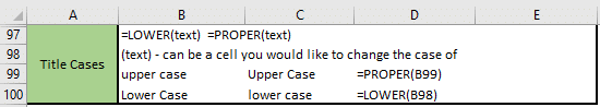
Let’s start with a nice easy one which helps with aesthetics. The Title Case functions will make all the words in a cell either upper or lower case. This would help if there is a regular report from a channel that doesn’t use upper case ” it can improve the look of a dashboard to have everything in the same case.
Dates
Knowledge Type: GTK
Excel Master Level: 1
Time Saved: 1-3 minutes per report
For those of us who never know today’s date (guilty!), Excel has a fix. Simply hold down CTRL and hit the “;” button and today’s date will automatically populate in the cell. This is a static date.
If a static date isn’t preferred, go ahead and use the =NOW() formula. When used in the chosen cell, it will populate a dynamic date and time (military) which updates when there is a change on the worksheet. When sharing a worksheet, this can help each user know when someone was last working on the sheet.
MROUND
Knowledge Type: Speed Racer
Excel Master Level: 2
Time Saved: 3 minutes per report
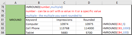
MROUND is a handy way to round your numbers to a specified multiple. This can really help to clean up data and make it easier to read, especially when working with very large numbers. We’ve also found ourselves using this when calculating budgets; generally round numbers are simply easier to work with.
Trim
Knowledge Type: GTK
Excel Master Level: 1
Time Saved: 2 minutes per report
Trim is a handy function that will eliminate spaces at the beginning or end of the chosen cell. Added spaces can prevent formulas from reading correctly. Simply use =TRIM(text) where (text) is the cell you need to trim. To see this and other awesome tips in action, check this out!
V/HLookups
Knowledge Type: HUGE TIME SAVER
Excel Master Level: 3
Time Saved: 5-60 minutes per report
VLOOKUP and HLOOKUP formulas are fantastic for pulling information out of large data sets and/or reorganizing information. See a tutorial here. Let’s say there is a report with a large amount of information needed regularly and in a specific order. Rather than reorganizing every single time, copying the list in the necessary order and writing an easy VLOOKUP to pull the data over can save time. Then the static data set simply needs to be copied over each time and the new data will populate in your VLOOKUPS in the correct order.
As noted below the visual, LOOKUP is a great alternative to VLOOKUP. As with most of Excel, there is more than one way to achieve the desired result. What it generally comes down to is usability and what you are most comfortable with. Vlookup needs to be read left to right (the lookup value has to be to the left of the column you are finding the answer in), and Hlookup reads top to bottom (the lookup value has to be above the row you are finding the answer in).
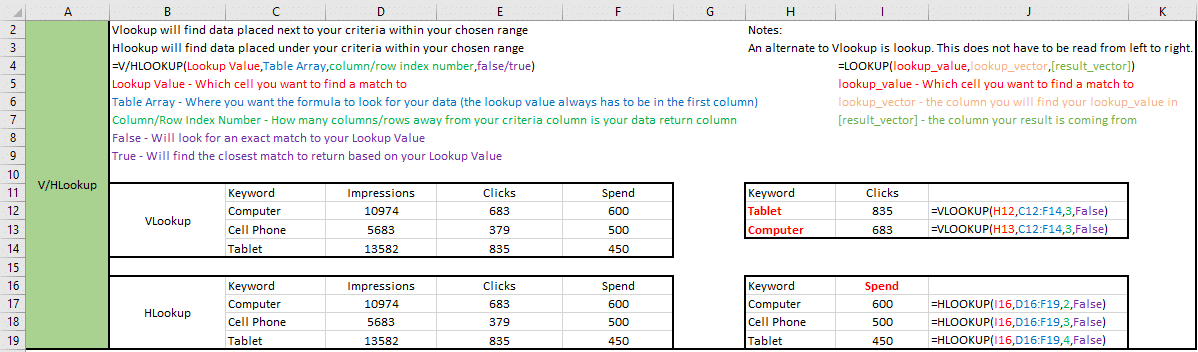
- =LOOKUP(lookup_value,lookup_
vector,[result_vector]) - lookup_value – Which cell you want to find a match to
- lookup_vector – the column you will find your lookup_value in
- [result_vector] – the column your result is coming from
Sumif, Countif, Averageif
Knowledge Type: Speed Racer
Excel Master Level: 2
Time Saved: 2-15 minutes per report
SUM, COUNT, and AVERAGE functions do exactly what they say. Put an “=” in front of any of those terms and they will add, count or find the average of whatever array of data chosen.
Take these one step further with SUMIF, COUNTIF, and AVERAGEIF. These formulas will return a result for your array, but will only look at the data that matches chosen criteria. For example, say we’re running a Twitter promotion with separate Campaigns ” each focusing on a device. A Twitter export automatically pulls by day, but we want to look at each campaign’s total. We can make a list of the Campaign names and use Sumif to add up all of the impressions for each Campaign. Then we need to know how many days it has been running, so we add a Countif and that will give us the number of days each Campaign has data for. On top of that, we want to see how many average impressions per day, so we use the Averageif to figure that one out.
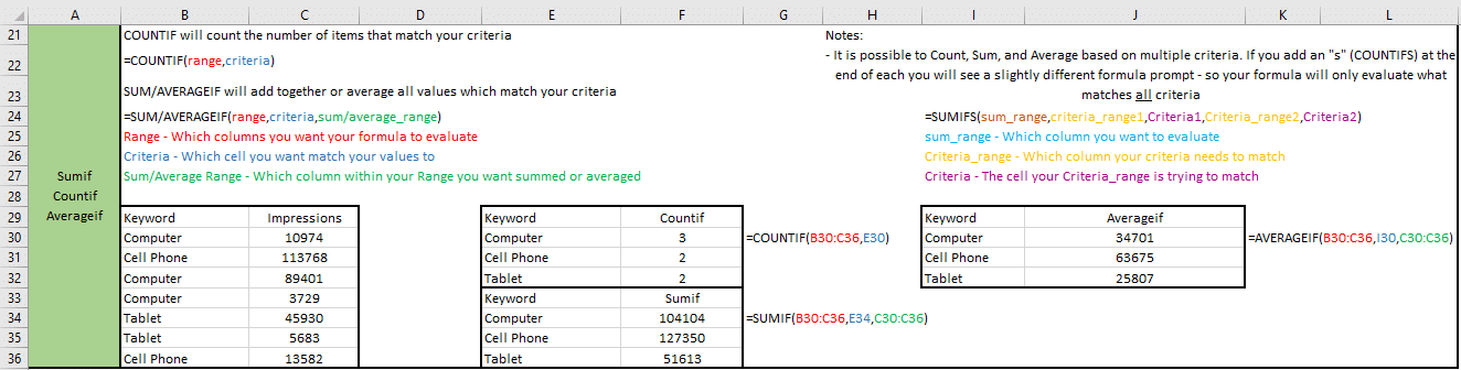
- =SUMIFS(sum_range,criteria_
range1,Criteria1,Criteria_ range2,Criteria2) - sum_range – Which column you want to evaluate
- Criteria_range – Which column your criteria needs to match
- Criteria – The cell your Criteria_range is trying to match
If/Then Statements
Knowledge Type: Amazing Multi-tool
Excel Master Level: 4
Time Saved: 5-60 minutes per report
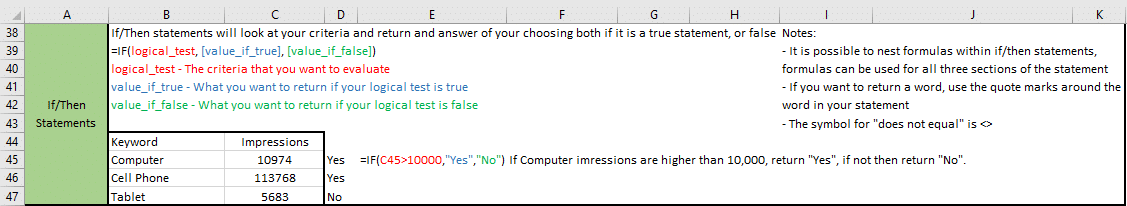
If/Then statements are really fun to play with (I mean, fun if you’re a nerd, like most of us… ) and the possibilities are nearly endless! This formula will look at specified criteria and return an answer depending on if the criteria is met (true) or not (false).
We use these constantly! For budget pacing we might set one up which will alert us with an “Over” or “Under” if the daily pacing falls outside certain thresholds. We have also used this when our data export contained “Active” and “Paused” campaigns; in that instance, we only wanted to run a formula if a campaign was labeled as “Active”. The formula read “=IF(cell=”Active”,(formula),”0″). So if the campaign was active, it would run the formula, if it was paused, it would input a zero. We also have it on good authority (from our in-house developers) that If/Then statements are basically like coding Java Script, so master these and you’re practically qualified to write website code!*
*Disclaimer: You will not actually be a developer, we were using hyperbole to prove a point. Happy “coding”!
IFERROR or IFNA
Knowledge Type: Must Have
Excel Master Level: 1
Time Saved: 3 minutes per report
Most of us use an IFERROR or IFNA qualifier on the vast majority of formulas. This will return a value of your choosing should your formula fail. It could fail because you have zeroes so it is trying to divide by zero; it could fail because you have blank spaces. There are any number of reasons why a formula can fail, but when it does, it will likely affect additional portions of your dashboard (even it if is just your total section). For this reason, a common choice of what to return in the case of an error is a zero; that way all of formulas will continue to function.

One very large caveat to keep in mind when adding this to formulas is to be cognizant of the data and how the formulas work, and to only use when you know why it could be returning an error. It can return, essentially, a false positive by negating an error which in some cases should be visible in order to fix.
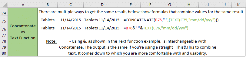
Text Function
Knowledge Type: Fantastic Multi-tool
Excel Master Level: 3
Time Saved: 1-10 minutes per report
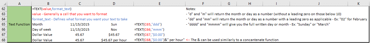
The Text Function has many, many uses. At the most basic definition, this function will turn a value (or cell) into the formatted text of your choosing. We have a few examples of uses shown, but go here for a more in-depth look at the options this function offers. We tend to use this most often to look at performance by day of the week or by month. In slightly more limited situations, it’s used to combine text and date into one cell and ensure the date is formatted as such.
Concatenate
Knowledge Type: Handy Dandy
Excel Master Level: 2
Time Saved: 2-5 minutes per report
Concatenate will combine the information from multiple cells or values into one string. One common way to use Concatenate is to pull two separate cells into one as a header. In the example below, we wanted to combine the Keyword with the Date so that it could be the header of our table. Rather than manually typing the values, we created a Concatenate formula which populates automatically whenever new information is pasted in.
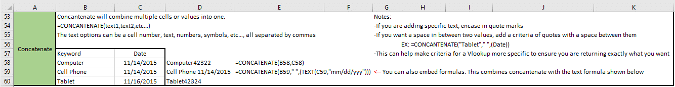
As you may have wondered, and was mentioned above, the & and Concatenate functions can generally be used interchangeably. We have had some trouble with the functionality of the & and tend to think that it can make a formula more confusing to read. The ampersand is a larger, more imposing symbol that gets in the way.
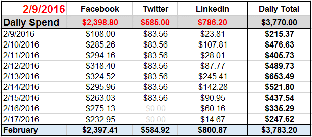
Dashboards
Knowledge Type: Moderate
Excel Master Level: 4
Time Saved: 5 minutes-hours (literally!) per report
These formulas can all be used on a one-off basis, but to really impress people and save a ton of time, the best course of action is to use these formulas to create Dashboards. When the same reports run over and over again, you can build a pretty report and pull all of your information in simply by updating your raw data. In this instance, we have a report where we pull spend and performance data from the social channels every morning. We take the raw exports and paste them into their tabs. Then, the formulas in our Dashboard pull all of the necessary information from each channel tab to compile it all into one report!
Designated tabs for each export:
![]()
Output:
We have reached the end of our nerdy Excel excitement for the day! We have but scratched the surface of the awesomeness that is Excel but these are the building blocks that will make anyone a reporting ninja! A few parting words of wisdom: With great power comes great responsibility. Practice due diligence; test, test, and test some more to ensure the formulas are pulling exactly what they are supposed to each and every time. Now go forth, test these out, and build an awesome report that will impress people!