We’re back with more tips and tricks for a faster, easier, more ninja-like approach to Excel! This time around the focus is on tips and tricks, rather than specific Excel formulas. We love Excel, this much is true. That said, sometimes it can be so frustrating and tedious that the thought of going Office Space on the computer might just cross our minds…
Replacing computers that often would be a drag, so instead, through some trial, error, and research, we’ve found workarounds and solutions for some common Excel annoyances.
Avoid Formula Overwrites
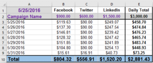
The bane of any spreadsheet owner’s existence is when someone overwrites a formula. While this isn’t 100 percent preventable unless cells are locked, one trick is to format all editable fields the same. For example, if all fields that people are allowed to change are Bolded and in a specific Colored font, it’s easy for anyone to identify where they can type without wiping out a formula. Also, always keep a master copy in a separate file so if someone DOES happen to jumble up the whole spreadsheet, there is a clean backup.
Conditional Formatting FTW
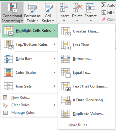
This can be found under the Home tab in Excel and is arguably one of the easiest ways to call out important information for speedy assessment. Conditional formatting is essentially an If/Then statement which formats a cell or array based on the criteria chosen. There are countless fantastic options for formatting that can really make a report pop and we highly suggest getting in there and playing around with them to uncover the full potential. Here are a few that we gravitate towards most often:
- Highlight Cells Rules The “Greater Than” function is used in a budget pacing document to highlight a channel when it has completed more than 50 percent of its allocated budget. In that same document, we have an If/Then formula which provides alerts if daily pacing is under or over for a timeline. The “Text that Contains” function highlights the cell if the If/Then formula does return with an “Over” or “Under” verdict.
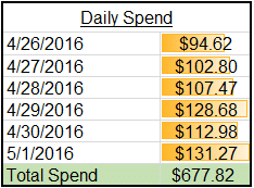
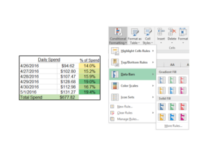
- Data Bars and Color Scales are two features that are geek-out-about worthy. They’re pretty colors that can really help tell a story and help the data stand out. The Data Bars add colored bars in the cells of your chosen data array, giving it an almost chart-like look highlighting the data as it compares to itself. The Color Scales option is exactly what it sounds like: It assigns a color scale going highest to lowest or lowest to highest.
Conditional Formatting
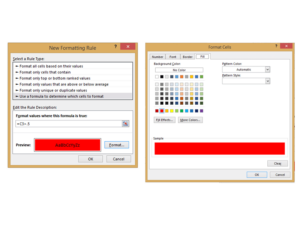
Another extremely useful tool within Conditional Formatting is the ability to format one cell based on the contents of a different cell. To do this, choose the “New Rule” option, then “Use a formula to determine which cells to format”. Once the chosen parameters are in the formula bar, click the “Format” button which opens a formatting screen with options for numbering format, font options, border options, and cell fill options. In one of our documents, the formula bar reads “=C3>50%” with the formatting chosen to highlight the formatted red if C3 is greater than 50 percent.
Format Painter
This handy dandy little tool utilizes the formatting from a chosen cell or array and applies it to another chosen cell or array. Found on the home tab, this takes the formatting – colors, number formats, underlines, size, etc. – and applies it to the chosen destination. Simply highlight the cell or array, click this button, then highlight an area the same size and the formatting will copy over. Double clicking this will allow the formatting to be used more than once.
Nesting Formulas
The ability to nest formulas within each other eliminates the necessity for multiple separate cells with different formulas in each, which eventually get combined in yet another cell.
-
- Begin with the most complex and build out from there. For example, in the following formula the final string is the most complex. By starting there, the sole focus is on the output produced by this portion, rather than on it being pulled in different directions by trying to decide how best to incorporate the rest of the requirements.
-
- If you are having trouble nesting multiple formulas, try building each component separately to ensure the desired output is produced, then combine.
- When writing a formula, click into the formula bar rather than the cell and it will color code the parenthesis, which makes it easier to ensure parenthesis are all enclosing the correct parts of the formula.
Anchoring Cells
When dragging a formula, the data set the formula is reading will change dynamically in whatever direction the formula is dragged. This can cause errors and/or a formula to read from the incorrect array of data. For example, for a formula counting A1:A23: If the formula is dragged down, the array will dynamically change to A2:A24, A3:A25, etc…; the formula is dragged to the right and the array will dynamically change to B1:B23, C1:C23, etc…
-
-
- If a formula is reading from a specific data set, anchoring the data set array in the formula is achieved by using the $ symbol.
- Any column letter or row number with a $ symbol in front of it will stay static when dragged and/or copied. The F4 key is the quick way to achieve this and will toggle between options if pushed multiple times.
- Anchoring an entire cell: $C$1
- Anchoring only a row: C$1
- Anchoring only a column: $C1
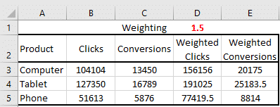
- For example, we want to multiply our metrics by 1.5 and want to drag the formula down and over so everything is calculating off of the same weighting (the formula in cell D3 would look like this): =B3*$D$1.
- When dragging from C3 down to C4&5 and over to E3-5, the first component (B3) will change dynamically as you drag, but D1 will stay static and will be multiplying both Clicks and Conversions by 1.5. With this formula in place, changing the 1.5 will automatically recalculate the cells formulating from it.
-
Dragging V/HLookups
When dragging one of these formulas, the third argument, which dictates the column or row the answer is returning from, will not change dynamically as it is dragged. If it needs to change dynamically, that change needs to be made manually. To override this, the argument dictating the column/row number needs to be directed to a cell which will change dynamically instead.
-
- In green, as the formula is dragged, B1 will become C1 and so on because it is not anchored (though row 1 could be anchored if the formula will be dragged down as well).
Various Ways for a Formula to Read Criteria
In a typical formula like the VLookup used above, your output will be based on a criteria cell. This can be limiting but there are a few workarounds:
- Instead of a criteria cell, a formula can look for text criteria. In the place of the criteria cell number we can write a word in quote marks “”Computer” ” and the formula will search your array for that exact text.
- If we are looking for a selection of text in a longer string, we add an asterisk inside the quote marks – “*Computer*”. Let’s say we have criteria in our array, such as Computer Mouse and Computer Keyboard, and want to add all items with the word Computer in it; the asterisks would achieve this.
- Similar to the previous example, we can use an & function to combine the quote marks and asterisks to cell criteria. For example, if we have the word Computer in cell B5 and want to read from that we would use the criteria “*”&B5&”*” and the formula will look for any items in our array containing the word Computer. This is helpful because rather than change the word in the actual formula, we can change the word in the cell and have it read correctly.
Quick Keys
Want to be a real Excel ninja? These are the keys (no pun intended)! With a few easy keystrokes, hunting down the right tab and tool can be eliminated almost entirely for the most common of actions.
-
- CTRL+Z/Y – Undo/Redo
- CTRL+C/V – Copy/Paste
- CTRL+B/U/I – Bold/Underline/Italics
- CTRL+PgUp/PgDn – Tabs between sheets in your workbook, PgUp moves backwards, PgDn moves forwards
- CTRL+F/H – Find/Replace
- Using Arrow Keys
- CTRL+Arrow Keys – Moves the active cell to the last/first cell in your data set in the chosen direction
- SHIFT+Arrow Keys – Selects cells one at a time in the direction of choice
- CTRL+SHIFT+Arrow Keys – Selects all cells in the given direction until it reaches an empty cell
- F2 – Activates edit mode for current cell
- ESC – Ends any active (edit mode) activity
- Number Formatting
- CTRL+SHIFT+1 – Number format with two decimal places
- CTRL+SHIFT+2 – Time format
- CTRL+SHIFT+3 – Date Format
- CTRL+SHIFT+4 – Dollar Format
- CTRL+SHIFT+5 – Percent Format
Oofta (that’s Minnesota speak for “Holy Crap!”). That was a lot of info we threw out there. Go test them out! Excel has a gold mine of efficient tips like these just waiting to be utilized by smart marketers! Wax on, wax off, Excel grasshopper.

